Lesson

51

Lesson Objective: In this lesson, we will learn how to create basic tables and show balloons.

TABLES vs. REPORT TABLES

In Pro/ENGINEER Drawing mode, there are two different types of tables that you can create.  They both start off the same way, but a report table takes it to the next level.  To clearly define the difference, we will first need to define some key terms:

Parameter – As we learned in Lesson 34 – Parameters and Relations, a parameter is used to capture data for the model that can then be used later for different purposes.  A good example of a user defined parameter is PART_NO.  This parameter is used to capture the part number of the object.  Typically, you would report this information on the title block in a drawing, and in Bill of Material tables.

Repeat Region – A repeat region is a grouping of table cells that gather information from the model, process it according to different rules set up by the user, and then reported back to the table in as many rows as it needs to accomplish the reporting.  A good example of a repeat region is one that gathers Bill of Material information from an assembly.  Depending on the type of information gathered, and what you want to output, the table can be as long as the number of models in the total assembly.

Report Symbol – A report symbol is a special parameter used in repeat regions.  It represents a full path to the location where data is stored.  For example, the PART_NO parameter that we talked about earlier is typically stored in the model (part and assembly files).  When the repeat region wants to extract this information from an assembly, the first thing it needs to know is how to get to this parameter.  In plain English, one might say that the PART_NO parameter resides in the model which is a member of the assembly.  In report symbol language, this would look like the following:

asm.mbr.part_no

Where asm represents Assembly, mbr represents Member, and part_no is the parameter that we are looking for.  There are hundreds of possible report symbol paths that can be used to pull data from models of varying types.

So, if you think back to a Bill of Materials table, as the repeat region starts to gather information, it goes from one component of the assembly to the next, gathering the value of Part_No for each model it encounters.  Some models are used more than once (screws, for example), so the value that it finds is duplicated, but counted.  When it is done gathering the values, it processes them.  We might set up a rule that we don’t want to have duplicate rows, therefore, when the output is created, for every value of Part_No that is identical, it tries to combine them into a single row of the table.

The more report symbols you have reported in your table (in separate columns), the better the chances are that there will be fewer identical rows created.  This helps in calculating quantities.  We will see all of this in more detail as we create a bill of material table in an upcoming example.

CREATING A TABLE

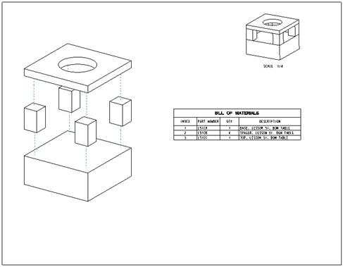
Since Report Tables and regular Tables start off the same, the first thing we’ll learn is how to create a table.  Therefore, we will open up the 51_BOM.drw drawing located in our working directory.  It looks like the following.

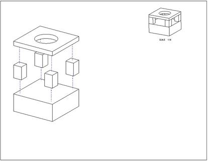
This is an assembly drawing (the model is 51_BOM.asm).  There are two views.  Both of these are general views.  One of them is showing an exploded state that was created in the assembly.  The other is a scaled isometric view to show what the assembly looks like together.

We are going to be creating a Bill of Materials table in the lower right of this drawing.

Building Rows and Columns

To start a table, we will go to Table, Insert, Table in the menu bar.  This will bring up the following menu.

At the top, we have two options: Descending and Ascending.  Descending means that the table is typically read from top to bottom, and any repeat regions that may expand in this table will expand downwards.  Ascending means that the table is typically read bottom-up, and any repeat regions will expand upwards.

Our BOM tables are typically Ascending, because they start just above the title block, and expand upwards.  For the purpose of this training guide, we will use the default of Descending.

The next section has two options as well: Rightward and Leftward.  Rightward means that we will read from left to right, and any two-dimensional repeat regions will expand out to the right.  Leftward means that we will read from right to left, and any two-dimensional repeat regions will expand out to the left.  We will talk about two-dimensional repeat regions later in this lesson.  For now, we will keep the default of Rightward.

The third section from the top contains two options also.  These are: By Num Chars and By Length.  By Num Chars means that the width and height of the cells we create will be based off of the number of characters of text that will fit exactly in that space.  By Length means that we will specify the actual length in the drawing units we use.  For example, we may want a cell to be 1.5” wide, and .25” tall.

The choice here really doesn’t matter, because most of the time we will adjust the actual width and height of the cells after the fact.  I do find it easier to use By Num Chars when defining the table initially, because there is fewer input needed.  Therefore, we will keep this default option.

We are now asked to start the upper left corner of the table (because of Descending, Rightward options).  We will pick out on the drawing to the right of the exploded view, and below the scaled general view.

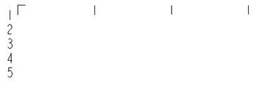
Once we pick the location for the upper left corner, we see the following.

The numbers across the top of this figure indicate the number of characters.  Each zero represents the next “tens” of characters.  The single vertical line at the left of this figure represents the left border of the first cell being created, as shown in the next figure.

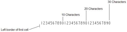
The purpose here is to pick on the number that represents the number of characters you want for the width of the column.  Personally, I pick at about the “10” location for each column I want to add just to do it fast.  Therefore, we will do the same.  Pick on the first 0 (or close to it) that you see in the line of numbers.  When we do, we see the following.

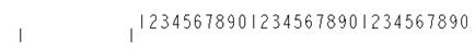
From this figure, we can see that we have defined our first column (left and right border).  Every “0” that we pick on from here adds one more column.  We want to have three columns in our table, therefore we will pick on the first 0 in this list, and then the first 0 of the next list of numbers, until we see the following.

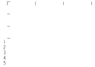
When we are done defining columns, we click on the middle mouse button.  This will cause the table definition to switch over to defining rows, as shown in the next figure.

Again, the numbers going down in the list represent the number of characters for the row height.   I like to pick on the 3 for each row I want to add.  We will add three rows, therefore, pick on 3 a total of three times to get the following.

We will click on the middle mouse button to finish defining rows once we have three created.  This will give us the table shown in the next figure.

We are now ready to start setting up the table.

Selecting Table Entities

We are going to take a moment to learn about selecting a table or selecting rows, columns or cells.  Start by clicking anywhere outside the table to make sure it is completely unselected.  Then, bring your mouse cursor just outside the upper left corner of the table.  When you do this, you should see the entire table highlight in blue, and if you wait a few seconds, a tool tip will appear, indicating that you are previewing the entire table, as shown in the next figure.

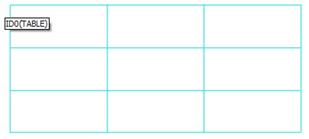
Selecting now will select the entire table, and then you would have the ability to perform any operation that can be done on the table as a whole, such as move or delete the table, rotate it, change the height and width of all cells simultaneously, etc.

This works for any of the corners, just by bringing your mouse to the corner itself.  If you place your mouse to the left or right of any row in the table, you will see the entire row highlight, as shown in the next figure.  NOTE: Your mouse must be outside of the table, or on the outer edge of that row.

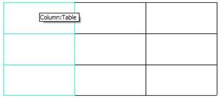
If you place your mouse just over or just below any column in the table, that column will highlight, as shown in the next figure.

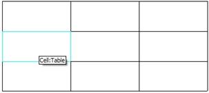
Finally, if you place your mouse cursor into the middle of any cell, just that cell highlights, as shown in the next figure.

Clicking with the left mouse button once you see the entity highlight will select that entity, whether it is the entire table, the row, the column or the cell.  To select multiple rows, columns or cells, use the Ctrl key.

Merge Cells

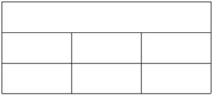
Before we start adding any text to the table, we should perform any merge cell operations.  We want to merge all of the cells in the top row into a single cell.  Therefore, we are going to select all three cells using the Ctrl key to do this.  Once you have all three cells selected, go to Table, Merge Cells.  Click outside of the table, and you will see the following.

We are now ready to add the static text to the table.

Entering Text (Static)

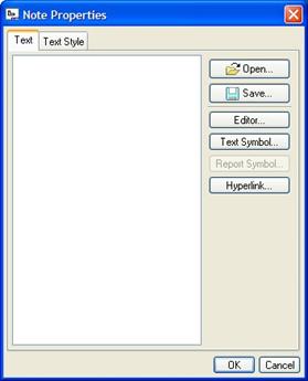
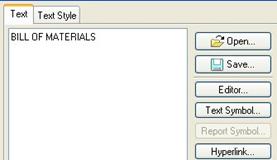
Static text is text that is not part of a repeat region.  Basically, all text not in a repeat region is going to be static text.  To add text to a table cell, double-click on that cell, which brings up the following properties window.

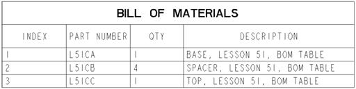
We will type in the following text in the large field provided: BILL OF MATERIALS, as shown in the next figure.

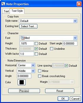
Next, click on the Text Style tab at the top.  When the text style window opens, make the following changes:

· Font = filled

· Text height = 0.1875

· Width Factor = 1.0

· Horizontal Justification = Center

· Vertical Justification = Middle

The following figure shows what this window should look like.

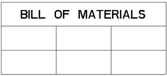
To see what the text will look like, click on the Preview button.  Click on OK to complete this text.  Our table now looks like the following:

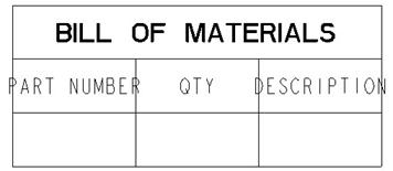
We will repeat this process to add text to each of the cells in the middle row.  The only text style change that we have to make for each cell is:

· Horizontal Justification = Center

· Vertical Justification = Middle

When done, your table now looks like the following.

Obviously our first and third columns are not wide enough – even for the titles.  We could fix this right now, but we still don’t know how much room our repeat region is going to need once it fills in with data, so it really is up to you whether you want to fix it now, or wait until later.

For practice, we will change it now, and probably again later.  To adjust the width of the first column, we first select the entire column (as discussed in the section Selecting Table Entities earlier).  Once we have the column selected, we right click and select Width.  This brings up the following window.

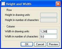
We can see that the Row fields are currently grayed out, because we selected a column.  We can change the width in the number of characters (currently 9) or the actual length (1.248” currently).  So you see, when we first started creating the table, it was easier to just pick random cell widths using By Num Char, because we can come in here later and specify exactly what we want.

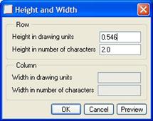
We will change the width of the column using the drawing units field with a value of 1.5”, and then click on OK.  Our table updates as follows.

Repeat this for the third column, and use a width of 3.0”.  The table will look like the following after this change.

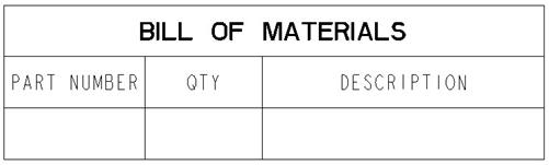
The only other change I might make at this time is to change the height of the last row (bottom) to 1 Character.  To do this, select the entire row, right click and select Height.  This will bring up the following window.

This time, since we only picked a row, the column fields are inactive.  We will change the 2.0 to 1.0.  Click on OK, and you will have the following table.

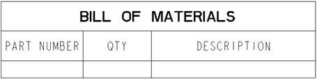
We are now ready to create a repeat region.  Save this drawing first.

REPEAT REGIONS

Not all tables that you create will have repeat regions.  In fact, most of the tables you create may only have static text in them.  The most common tables with repeat regions that I have created or have seen created are:

· Bill of Material Tables

· Pipe/Cable Cut-Length Tables

· Part Parameter Tables

· Family Table Driven Tables (Two-Dimensional)

· Miscellaneous Manufacturing-Mode Tables

By contrast, all of the tables in the drawing formats are tables with static text.  Some of the static text actually pulls value from part, assembly or drawing parameters, but does not belong to a repeat region.

Creating A Repeat Region

There are two ways to create a repeat region.  The first is to select a row, and then right click and select Add Repeat Region.  The second method is to go to Table, Repeat Region, and then select Add from the menu manager that appears.

We will do the latter of these two, since most of the other Repeat Region functionality is through the menu manager.  Therefore, go to Table, Repeat Region.  This brings up the following menu.

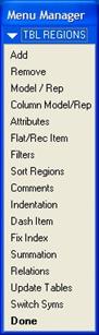
To add a repeat region to a table that currently does not have one, we would use Add.  when we click on this option, we get the following sub-menu:

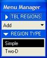
Simple is used to create most repeat regions.  Two-D is only used to create two-dimensional repeat regions.  We will have a completely different section devoted to two-dimensional repeat regions, so for now, we will click on Simple (which is already the default).

In the message bar, we get the following prompt: “Locate corners of the region.”  We are supposed to pick the first and last cells that make up the region in a row.  Therefore, we will click on the following.

NOTE: You do not need to hold down the Ctrl key for this.  When you select both cells, the only way you’ll know that you successfully created the region will be the following message bar statement: “Region has been successfully created.”

To verify that a region exists, we will go to the TBL MANAGER table, and select on the Switch Syms command.  If we have a repeat region in our table, the region will outline in green, as shown in the next figure.

The Switch Syms command is used to let you get back to the report symbol names once you add them to the table to see what they are.  We will see this soon.  For now, just remember that it is the way to see into the repeat region.  We will click on Switch Syms once more to go back to the table view (the green outline should disappear).

Removing Repeat Regions

Had we needed to remove a repeat region from our table, you would go to Table, Repeat Region, and then select Remove from the menu manager.  We will leave our repeat region in our table.

Adding Report Symbols

The method to add a report symbol to our repeat region cell is the same as entering static text, but the result is quite different.  Therefore, double click in the first cell of the repeat region.  When we do this, we see the following.

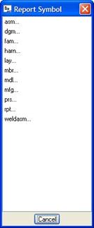
The way this works is that you select a category for the first screen.  For example, if you were adding a parameter from the model to fill in a Bill of Materials table, (PART_NO, for example), you would select asm in this first screen.

Once you select a category, the screen updates to show only additional sub-categories that are related to the first one you picked.  We will pick on asm first, and our window updates as follows.

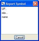
On this window, we can see three options.  The first one, labeled UP, takes you back to the previous screen (in case you made a mistake).  We then have mbr and name to choose from.

One other thing to point out is that one of the options has three dots (periods) following it, while the other one does not.  Any symbol that has dots means that there are further sub-options for this selection.  In this case, name does not go any further.  In case you are wondering, asm.name would report back the name of the top level assembly, which for a bill of materials table doesn’t do much for us.

Therefore, we will click on mbr…, which brings up the next set of options.

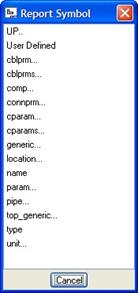
We can see that there are a lot of options at the assembly member level.  There are a few to point out here.  First, the name option doesn’t go any further.  Asm.mbr.name will give back the actual file name for the model in the assembly.  This might be useful if the name used for the part is the same as the part number parameter.  Often, this is not the case (especially for inseperable assemblies).

Type also does not go any further.  Asm.mbr.type would give back the type of file it is (PART, ASSEMBLY, BULK-ITEM, etc.)

The third one that doesn’t go any further is User Defined.  User Defined allows you to type in a value for the last symbol.  This is what we use for capturing model parameters (PART_NO, for example).  Therefore, if we select on User Defined, the message bar prompts for the name of the symbol text we want to enter.  We will type in PART_NO, as shown in the next figure.

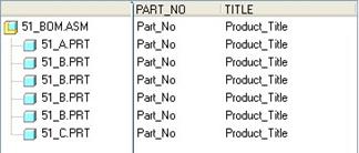
When we click on the <ENTER> key, we will see the following in our table.

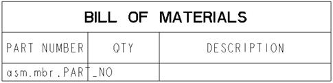
We will continue this same process by double-clicking on the last two cells and entering the following:

· Second cell – rpt.qty

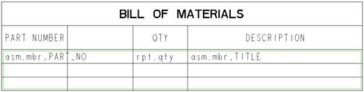
· Last cell – asm.mbr.TITLE (NOTE: Use the User Defined option, and type in TITLE)

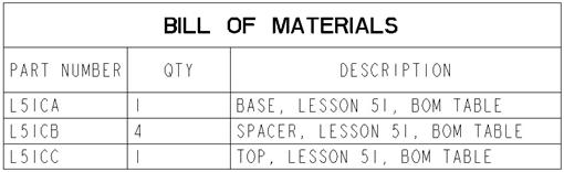
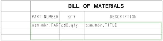
Rpt.qty will give us the reported quantity.  We will describe how this works soon.  asm.mbr.TITLE will give us the description of the part by using the TITLE parameter in the model.  The table should look like the following when these two cells are done.

Don’t worry about the fact that the first report symbol (asm.mbr.PART_NO) doesn’t completely fit inside the cell.  The actual value that is reported from the parameter is what we care about, not the entire path to that value.

To see the actual values from the model, we need to update the repeat region.  To do this, go to Table, Repeat Region, Update Tables.  When we do this, we see the following.

Do you know what is going on here?  Unfortunately, the PART_NO and TITLE parameters were never filled in for the models.  Therefore, their default values are reporting, and are all identical.  We have no idea which row represents what component on the assembly.

This is why it is critical to fill in parameter information in the model.  Therefore, we will have to go do this.

MODIFYING PARAMETERS

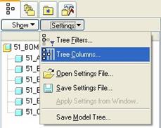
The easiest, and fastest way to do this will be to open up the assembly model itself.  Once you have the 51_BOM.asm assembly open, we are going to focus on the model tree.  At the top of the model tree, pick on Settings, Tree Columns, as shown in the next figure.

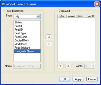
This brings up the following window.

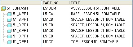
Using the Type pull-down menu, select Model Params, and then add PART_NO and TITLE to the list on the left, as shown in the next figure.

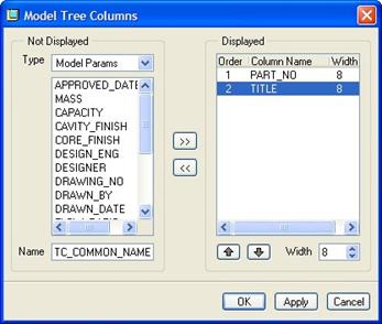
Click on OK, and your model tree will update as follows.

Now, we can click on the value in  the PART_NO and TITLE columns and edit the value.  We will type in the following parameter values for each part and the top level assembly.

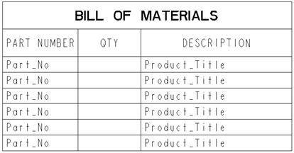
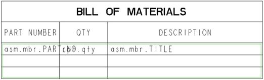
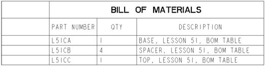
Save the assembly, and return to the drawing, which should now show the updated table, as we can see in the next figure.

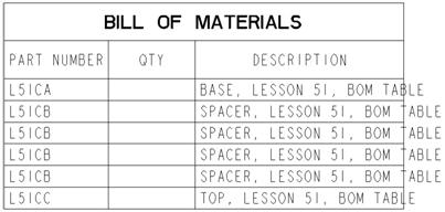
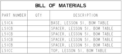
Now we can see that our DESCRIPTION column is not wide enough to accommodate the values.  We will change the width of this column to 4.0 inches, and our table now looks like the following.

We are getting close to a completed table.  There are some attributes we should set to get the table to be completed.

Repeat Region Attributes

Go to Table, Repeat Region, Attributes, and pick on the repeat region in the table.  This brings up the following menu.

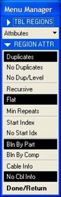
In the first section, we see the following options:

· Duplicates – Allows multiple rows with the same data to exist.  This is why we see several rows that look identical to each other.  Unfortunately, Duplicates will not show a quantity in the quantity column (which is why we don’t see any right now).

· No Duplicates – Does not allow duplicate rows to exist in the table.  For any two or more rows that are the same, the repeat region will calculate the total number of these rows and report that quantity in the second column.

· No Dup/Level – Does not allow duplicate rows to exist for each level of the assembly.  This option only works if you have your level reporting set to Recursive.

The second section is used to identify the level of the assembly reported.  The options are:

· Recursive – Shows all levels of the assembly, including the assembly itself.  Sub-assemblies will show all of their components on the table as well.

· Flat – Only reports the items at the top level of the current assembly.

The next option, Min Repeats, allows you to specify the minimum number of repetitious rows allowed in the repeat region.  The default is 1, which will allow for blank lines to appear if data is missing from certain components.  I recommend keeping this setting at 1 unless you have an advanced table function you are trying to work with that requires the number to be set to something else.

The following section deals with indexing numbers.  The options are:

· Start Index – Allows you to specify the number that the repeat region starts at when indexing rows.

· No Start Idx – Always starts the numbering at “1”.

In the next section, we see the following two BOM Balloon options:

· Bln By Part - When you suppress or replace a component to which a BOM balloon is attached, this command reattaches the balloon to another placement of the same part.  If no other copy of the part exists in the assembly, then the BOM balloon disappears from the drawing.

· Bln By Comp – Specifies that simple BOM balloons reattach themselves to whatever component replaced the one that originally owned the BOM balloon.

The last section deals with Electrical Cable reporting.  Since we don’t use this module, we will not go over this section.

For our table, we will set the attributes to No Duplicates, Flat, and Bln By Part.  When we select these options, and then click on Done/Return, the table updates to the following.

We can see the quantity field has now updated to show the quantities.  Again, keep in mind that the quantity field (rpt.qty), will report the total number of rows that contain the identical information.  If we were to change the PART_NO parameter and TITLE parameter values for the 51_A component to match those of the 51_B component, then we would see one row with a quantity of 5 instead of 4.  So this quantity is only as accurate as your parameter information.

The good news is that we can assemble in two models that (for one reason or another) had to be modeled as separate parts but they represent the same part.  By making their parameter information identical, the BOM table will report 2 for the quantity instead of two separate lines.

To go back and see the report symbols that were used in this table, we would click on Switch Syms again, and we would see the following.

We can still see all three rows, but only the first row shows values (the report symbols that we used).  Click on Switch Syms again to get back to the parameter values.

ADDING ROWS/COLUMNS

One column that we typically show in BOM tables is an indexing number that is used to correlate to BOM balloons.  Unfortunately, we do not have one in our table right now.

To add a column to our table, we go to Table, Insert, Column, and then pick close to the side of the cell where we want to add the column.  If we pick toward the left side, it adds a column before the one we picked in.  If we pick toward the right side, it adds a column after the one we picked in.

The index column typically comes first in the table, so we would want to pick in the following location.

When we do this, a column is indeed added to our table, as shown in the next figure.

Unfortunately, if we use the Switch Syms command, we can see that our repeat region was not expanded into the new column.

Therefore, we will delete this column that we just added.  Click on Done from the repeat region menu.  Select this column, and then hit the delete key.  We get the following warning.

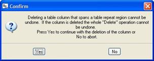
You will get this message because a repeat region exists in the table, not because we actually do span a repeat region.  So we will click on Yes, and our column is now gone.

Therefore, we will have to do something else to get the column into the table.  We will go to Table, Insert, Column again, and this time pick on the following location.

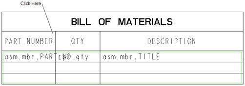
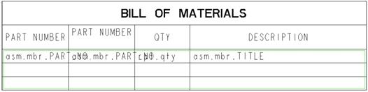
The column is now added in between PART NUMBER and QTY, as shown in the next figure.

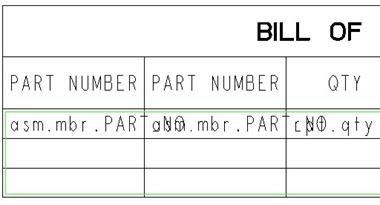
The good news is that our repeat region does span the entire table, and we can now cut and paste the text from the first column into the second.  To do this, we will click once on the cell containing the static text “PART NUMBER”.  While this cell is highlighted, click on Ctrl-C (Edit, Copy) and then click into the empty cell to the right of it, and press Ctrl-V (Edit, Paste).  The text appears in the second cell, as shown below.

We will do the same for the report symbol in the next row, giving us the following.

Now, we can go in and edit the text style to justify them like the originals, as we can see in the next figure.

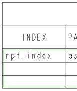
The last thing we need to do is edit the text in the first column.  For both cells, double-click and enter the appropriate values: INDEX for the static text cell, and rpt.index for the repeat region report sym cell.  The following figure shows the table when changed.

Now, go back to Table, Repeat Region, Switch Syms, which will give us the following.

On your own, center justify the report symbols for the INDEX and QTY columns.  HINT: You only need to do it for the cell that contains the report symbol, and all other filled in cells will get the same result.  The table will look like the following with the justification.

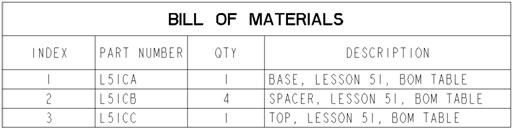
At this time, our drawing should now have a completed bill of material table, as shown in the next figure.

Save the drawing.

BOM BALLOONS

In Drawing mode, there are two types of balloons you can show/create.  On the drawing toolbar, there is a balloon note.  This is nothing more than a balloon symbol with variable text that you manually input. 

The other type is tied to repeat regions, and fills in automatically from the BOM table.  You can show these balloons on the views automatically, just like dimensions, and then clean them up.

I always recommend using the automatic balloons for linking to BOM tables instead of creating balloon notes.

Showing BOM Balloons

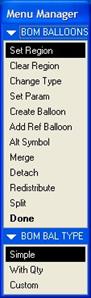
We are going to continue to work with the same drawing (51_BOM.drw).  From the menu bar, select Table, BOM Balloons.  This brings up the following menu.

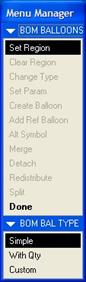
At this time, we need to identify what type of balloon we want to use.  There are three choices:

· Simple – Creates a circular balloon that only lists the index number.  You have the ability to report any report symbol in the balloon, but no quantity is shown.

· With Qty – Creates a circular balloon that lists the index number and quantity.  The index number can be replaced with any other report symbols in your table.

· Custom – Can use any custom symbol you have defined as long as it as either \index\ or \index\ and \qty\ defined as variable text.  This would allow you to create a balloon that was oblong in shape, or oval, or a star, etc.

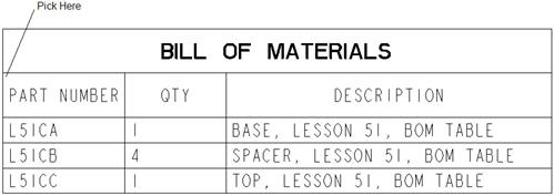
To start, we will select Simple, and then pick on the repeat region in the table.  NOTE: You need to pick what type of balloon you are going to use BEFORE you select the repeat region.  If you pick the repeat region first, it takes whatever value is highlighted in the bottom section (which is usually Simple by default).

Now that we have picked the repeat region, the rest of the menu options become available, as shown in the next figure.

We will now click on Create Balloon, which brings up the next menu.

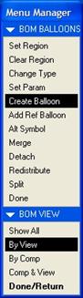
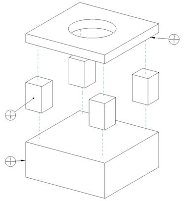
We can show balloons by view, by component, or by component and view, or we can simply show all balloons.  Since we will only have three balloons (one for each row in the BOM table), we will click on Show All.  When we do this, the three balloons appear on the drawing, as shown in the next figure.

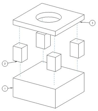
We can see that the shape is a circle, and there is an indexing number that corresponds directly with the index number in the BOM table.  These balloons are directly linked to the table.  If we were to sort the table differently from how it is now, the index numbers would change to match the table.

Edit Attachment for Balloons

By default, the balloons are going to appear on the drawing view where you can clearly see the component that the balloon references.  In this case, all three balloons went to the larger exploded view – which is perfect for what we need.

The default attachment type is a leader with an arrow head that points to an edge on the component that represents the row the balloon is tied to.  You can not change a balloon reference to point to a different component than what it currently belongs to.  This is not true with balloon notes, which have no intelligence.

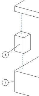
For example, component “1” and component “3” only exist once in the assembly.  The balloons for these can only touch edges or surfaces for the single models in the drawing view.

Component “2” however is used four times in the assembly.  Therefore, it could be attached to any one of the four components on the drawing view.

We will show how to change the entity to which the balloon references.  To do this, first select the balloon with the “2” in it.  When it highlights in red, use the right mouse button to select Edit Attachment.  This is shown in the next figure.

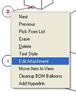
This will bring up a familiar menu that we saw when placing notes on the drawing.

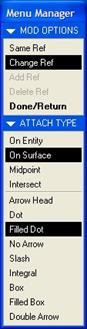
We will select the On Surface and Filled Dot options, as shown above, and then pick out in the middle of the surface that the balloon is currently touching.  Click on Done/Return, and refresh your window to see the following.

Typically, you should use an arrow head when pointing to an edge, axis, vertex, or datum curve.  Use a filled dot when pointing out in the middle of a surface.

Clear Region

If you want to remove all balloons from a drawing, the easiest, and preferred method is to clear the region.  We are not going to do this, but if you did want to – you would use Table, BOM Balloons, Clear Region, and then pick on the repeat region.  You will get a prompt to clear the region.

Change Type

We want to use a With Qty balloon instead of a simple.  To change all balloons over to a different type, we use Table, BOM Balloons, Change Type, and then pick on the repeat region.  This brings back up the menu with the three types: Simple, With Qty, and Custom. 

We will pick on With Qty, followed by Done/Return.  The balloons will change to look like the following.

In this symbol, there are two numbers.  The number on top is the index number.  The number on the bottom is the quantity.  We can see that the balloon for item “2” shows a quantity of “4”.

Split

When you have quantity balloons, any balloon that is reporting more than a quantity of “1” can be split up.  This is extremely common for fasteners or library-type items that may be used all over your assembly, and in sub-assemblies.

We will demonstrate this with a simple example.  We can split up the quantity balloon for component “2”, because our quantity is “4”.  We can not split up the balloon for components “1” or “3”, because they only have a quantity of 1.

To split the balloon, go to Table, BOM Balloons, Split, and then pick on the balloon to split.  We will pick on the component “2” balloon.  When we do this, we get the following prompt in the message bar: “Enter amount [Quit]”.  We will enter 1 and then hit the <ENTER> key.

We are now asked to pick the location on a different instance of this component, and we will pick in the following location.

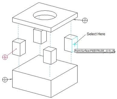
The surface will become selected, and we will use the middle mouse button to locate the balloon out to the location where the “Select Here” note is in the figure above.  Our completed balloon is shown in the next figure.

We can see that the new balloon contains only the quantity that we specified (1), which is subtracted from the original balloon (4-1=3).  We can now edit the attachment for this new balloon to select Filled Dot, to get the following.

Save the drawing.

Merge

The opposite of splitting up a balloon is to merge a balloon.  When you merge two quantity balloons together one of two things will happen:

· If the two balloons represent the same component, a single balloon will result with the sum of the two quantities.

· If the two balloons represent different components, the one that is merging with the other will attach itself to the outside of the other, and its leader will disappear.

We will demonstrate both of these.

Same Component Merge

We will start by going to Table, BOM Balloons, Merge.  In the message bar, we get the following prompt: “Select quantity balloon to be merged.”  We will pick on the component “2” balloon that has a quantity of “1”.  Once we pick this, we get the following prompt: “Select quantity balloon to be merged onto.”  We will pick on the other component “2” balloon with a quantity of “3”.  When we do this, only one balloon remains, with a quantity of “4”, as shown in the next figure.

Different Component Merge

Now, we will go to Table, BOM Balloons, Merge, and for the first balloon, pick on the component “3” balloon.  For the second balloon, pick on the component “1” balloon.  We will get the following result.

We can see that the component “3” balloon attached itself to the side of the component “1” balloon.  If we drag around the “1” balloon, “3” moves with it.

When do you typically use something like this?  Suppose you are mounting a plate that gets fastened down with four hex head machine screws, four lock washers, four flat washers, and four lock nuts.  Instead of showing balloons for the plate, the screw, the washer, the lock washer, and the nut, having leaders going all over the place, it is cleaner to show the balloon for the plate with the leader, and then merge the rest of the balloons to this one.  Doing this sort of “implies” that the hardware is tied to the plate, and also helps in the assembly of the plate.

Another good usage is if it is part of a kit that came with these different (but separate) components.  By merging the balloons together, you can imply that they are all together, possibly even before they are assembled together into the top level assembly.

Save and close this drawing.

TWO-DIMENSIONAL REPEAT REGIONS

In this section, we will learn about two-dimensional repeat regions.  If you recall from our repeat region tables before, our regions expanded in a single direction.  A 2D Repeat region expands in two directions.  The most common type of 2D repeat region is a family table driven table.

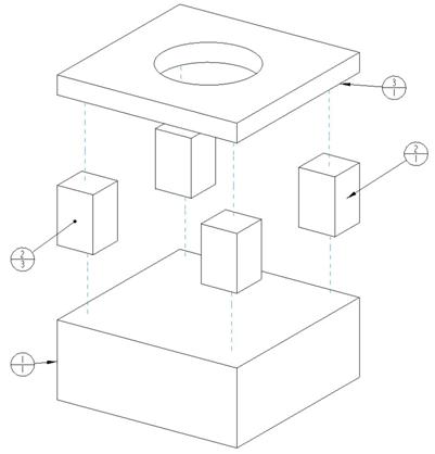
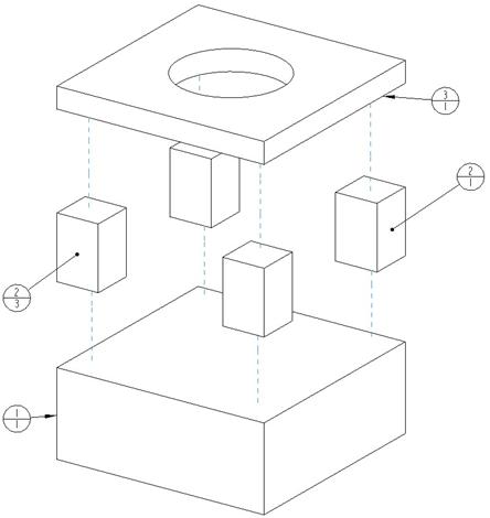
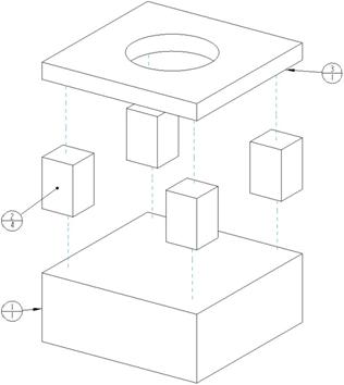
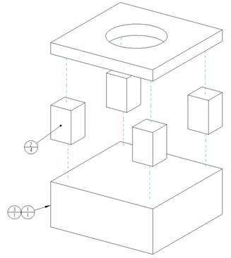
To demonstrate this, we will open up the 2D_Rpt_Region.drw drawing, which initially looks like the following.

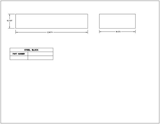
This drawing will be a tabulated drawing for a family table of steel blocks of varying sizes.  As we learned in Lesson 35 – Family Tables, there is some preparation that is done to the model to get it ready for a family table.

This model has three dimensions: LENGTH, WIDTH, and HEIGHT.  It also has parameters.  Our family table has all of these dimensions as varying items, and we also have the TITLE parameter to capture the different descriptions for the individual sizes.

We went ahead and modified the dimension symbol names to their respective titles (LENGTH, WIDTH, and HEIGHT).  We then created the family table and added these three dimensions, followed by the TITLE parameter.  The family table was then verified to make sure all instances are working.

On the drawing, we added two views, and we are showing the dimensions for the block.  We went into the properties for these dimensions, and changed the display from “@D”, which displays dimensional values, to @S, which displays the symbolic name for the dimension.  That is why you can see “LENGTH”, “WIDTH” and “HEIGHT” on the drawing views.

Then, we created a simple 2-column, 3-row table, and merged the two cells together in the first row.  We added some static text in the first row, and in the first cell of the second row.  The last thing that was done was to justify the text in the cells.  I took the liberty of adjusting the text justification in the empty cells as well, because I know what the final result will look like, and I wanted to clean it up ahead of time.

Creating the 2D Repeat Region

We will now go to Table, Repeat Region, Add.  In the lower section of the menu manager, we will select Two-D.  We get the following prompt in the message bar: “Locate corners of the outer boundary of the two-dimensional region.”

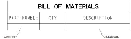
We will pick on two cells that define the upper left corner and lower right corner of the region we are creating.  Therefore pick the cells in this order:

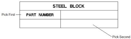
NOTE: If your table were ascending and/or leftward, the order of selecting the corners would be different.

Once we pick the second cell, we get the following prompt: “Select a cell to set the upper border of the row & column subregions.”  This time, we have to pick the cell that is going to be expanding in two directions simultaneously.  If you imagine that the last cell in the second row only expands to the right, and the first cell in the third row only expands down, then the cell in the lower right corner of the table (the one that is labeled “Pick Second” in the figure above) is the one that expands both down and to the right.

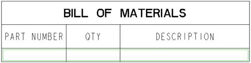
Therefore, we will pick on the cell in the lower right corner of the table.  When we do this, we get the following confirmation: “Region has been successfully created.”  Click on Done to complete the definition of this region.

We will now go to Table, Repeat Region, Switch Syms, and we see the following.

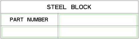
We can see a single green rectangle that goes around all four cells.  Then, we have a rectangle that just goes through the last row, and another rectangle that goes through the last column.

We will now add our report symbols.

Report Symbols

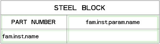
Double-click on the second cell in the second row, and use the following report symbol path: fam.inst.param.name, as shown in the next figure.

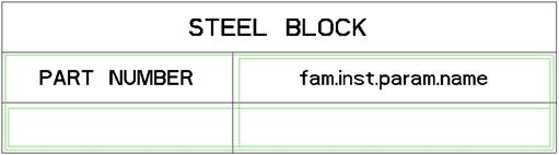
This report symbol will take the parameter name from the family table instances (such as LENGTH, WIDTH, HEIGHT and TITLE) and add them as columns to the table.  Notice how this text is already centered and is in a bold (filled) style?

Now, double-click on the first cell in the last row, and add fam.inst.name to this cell, as shown in the next figure.

This report symbol will show the family table instance names and report them as rows in the family table.  Again, we have already left justified this text, and made it bold.

The last cell will contain the fam.inst.param.value report symbol, as shown in the next figure.

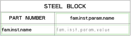
This report symbol will show the value for the parameter (LENGTH, for example) for each instance in the family table.  Therefore, this will report as the columns are added, and as the rows are added.

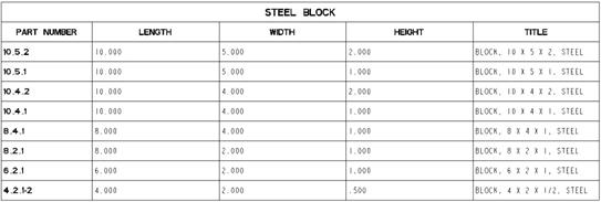
If we now go to Table, Repeat Region, Switch Syms, we will see our expanded table.

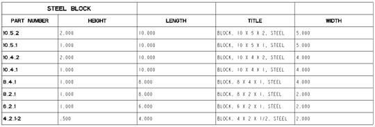
There are a few things to point out that we will need to address.  The first is that our header row isn’t merged all the way across.  Therefore, we will need to pick on each cell (while holding down the Ctrl key), and then go to Table, Merge Cells.  This will fix this, as shown in the next figure.

The second thing to point out is that all of our columns (starting with the HEIGHT column) are all the same length.  We can not change this.  Because the original table didn’t have all of these columns, it takes its width from the last one in the repeat region.  We had to make the column wide enough to accommodate the TITLE column, which meant that all the rest of our cells are large compared to their data.

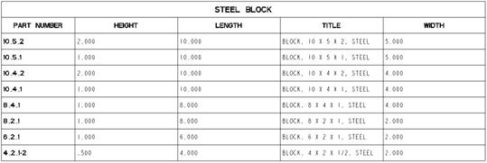
The last thing to note is that the columns (starting with HEIGHT) are in alphabetic order.  This is okay, except that we might want to show the WIDTH right after the other dimensional columns.  When we create our family table, we add dimensions and parameters in a particular order (or at least we should).  The order in the family table itself can be shown on the drawing by going to Table, Repeat Region, Sort Regions, and then pick on the repeat region. This brings up the following menu.

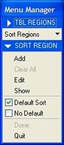
To create your own sorting, you would click on Add and then define the type of sort (ascending or descending), and then pick on the cell to sort by.  There is a Default Sort, which is already selected.  This default sort is what is currently controlling our table.  We also can see an option called No Default, which will show the table columns in the same order as they appeared in the family table itself.  We will click on this option, followed by Done, which will make our table appear the way we want it.

Save and close this drawing.

LESSON SUMMARY

Tables are used frequently in drawing mode, especially for assembly drawings where Bills of Materials are common.  Take advantage of repeat regions to make your tables dynamic.

You can save out your tables and retrieve them in later.  The report symbols in the tables will automatically read from whatever model is currently active at the time the table is created or updated.

Use BOM Balloons in conjunction with BOM Tables to get the maximum automation out of your drawings.

There is a lot more functionality with Report Tables and Balloons that wasn’t covered in this fundamentals course.  Feel free to contact your CAD Administrator to learn more.

EXERCISES

None