Lesson

220

Lesson Objective: In this lesson, we will learn about the Boundary Blended Surface tool.

BOUNDARY BLEND SURFACE USAGE

None of the tools that we have used so far would help you take boundary curves to define a surface, and internal curves to control the shape across the boundaries.  This is what a boundary blended surface is all about.

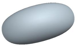
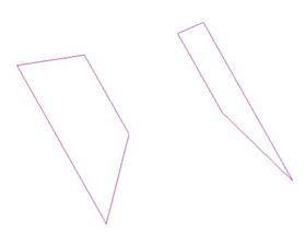
To demonstrate this, we will open up the following part (Boundary1.prt)

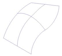
We are going to create a new surface by blending the outside curves together, but using the internal curves to define the shape.

DIRECTION CURVES

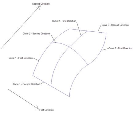
When you define boundary blend surfaces, you define curves or edges in one or two directions.  It doesn’t matter what you consider the first or second direction, as long as you keep track of it yourself.

In our example, we are going to consider the following directions, and curves in those directions.

CREATING THE SURFACE

To create a Boundary Blended Surface, click on the following icon in the feature toolbar.

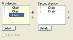
The dashboard for this feature looks like the following figure. The fields at the bottom are not labeled, but they are used to pick curves in the first, second and approximate directions.

The first direction curve field is currently highlighted in yellow, meaning that it is active.  We will select the first and third curve in the first direction, as shown below.  NOTE: Use the Ctrl key to select both of these.

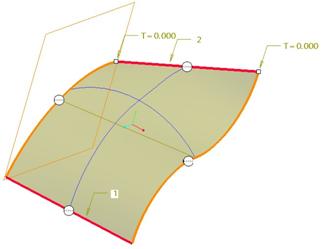
Once we select these, the first field at the bottom will say 2 Chains.  We can see a plane highlighted, and we can also see two circles with little symbols in them.  We will discuss what these mean a little later.

Now, we will click in the second direction field, and select the first and third curves in this direction, as shown in the figure at the top of the next.

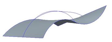
If we look at a full preview, and rotate the model, we can see that our surface does not intersect the two curves in the middle of the part, as shown below.

Click on the full preview button again to return to the feature definition.  We are going to pick on the Curves slide-up panel.  It will look like the following.

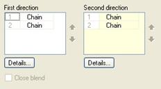
As you can tell, this panel is used to define the first and second direction curves.  Currently, we are active in the second direction, so we will pick in the first field to activate first direction curves. We are going to hold down the Ctrl key and pick on the second curve in the first direction.  It will appear in this panel as the third chain on the list.

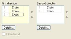
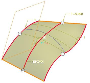
On the model, the dynamic preview has disappeared, because it can not build the surface in the order the curves were picked.  We need to move the new curve to the middle of the list so it acts as if we picked it second instead of last.  To do this, we will select on the 3 Chain item so it becomes highlighted, then select the up arrow that appears, as shown below.

As soon as we do this, the dynamic preview appears again, as shown below.

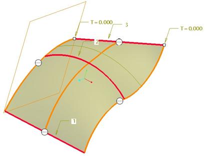
Now, repeat this process for the second direction curves.  We are going to hold down the Ctrl key and select the middle curve in the second direction, then repeat the process of moving it up the list so it becomes the second curve listed.  When we do this, we can see the preview for the final surface, shown at the top of the next page.

We will now accept this surface, and it will look like the following.

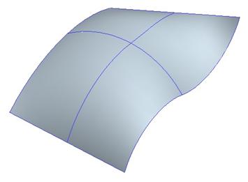
If you rotate the model, you will find that it goes through all of the curves.

EDGE ALIGNMENT AND ADVANCED OPTIONS

One of the more common options you will adjust in boundary blended surfaces is edge alignment (boundary conditions) and advanced options (edge influence).  To demonstrate this, open up the Boundary2.prt part file.  It will look like the following.

Constraints

If you recall from the last section, on each selected boundary curve, there is a white circle with markings in it.  These circles are used to identify and define the boundary conditions (constraints) that exist.  There are four possible constraints to choose from.  They are shown in the following figure.

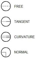
When selecting constraints, you should be aware which surface(s) is being referenced, as it will determine whether the condition can be satisfied.

In our current model, we are going to create a surface that will connect these two sides and then adjust boundary conditions to get the final result.  To do this, we will go back into our boundary blended surface.  For the first direction curves, we will pick the top edges of each side, as shown below.

We don’t have any side curves to define a second direction, but that is okay.  The problem that we have right now is that it is a flat surface connecting the two edges that we selected.  We actually want the surface to be tangent to the existing surfaces.  Therefore, we will define edge alignment (or boundary conditions). 

When we click on the Constraints slide-up panel, we see the following.

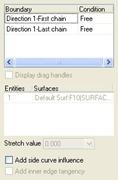
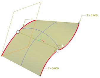
It lists the first and last curves/edges selected in the first direction.  Currently, the boundary condition at both of these sides is “Free” or in other words, no condition is set.  When we pick on one of the edges in the panel, the adjacent surface highlights in an orange outline, as shown in the following figure.

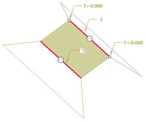
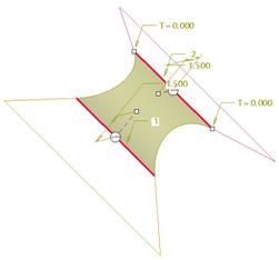
We are going to change, for both edges, the boundary condition from Free to Tangent as shown below.  We can do this directly in the slide-up panel, or by right-clicking on the circle on the model.

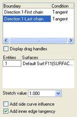
The surface to which the boundary surface assumes tangency will be listed in the field below.  In many cases, it will assume a surface that shares the edge selected, so we won’t have to change anything in this field, but you will want to verify this.  As soon as we set the tangent conditions for both edges, click on the “Display drag handles” check box, and our dynamic preview will update to show the result.

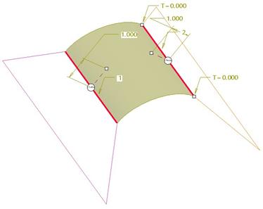
For each of the tangencies defined, there is a dimension that appears on the model.  This dimension determines how far from the edge into the surface does the tangency exist.  The larger the number, the more domed the surface will be.  The smaller the number, the flatter the surface will be.

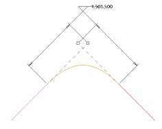
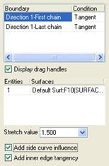
We will change these values to both be 1.5, which gives us a nice dome, as we can see from the side.

SIDE CURVE INFLUENCE

Now that we have a nice dome to our surface, we can still see that it looks a little strange.  We don’t have a tangency condition with the sides of the original surfaces.  This is really evident from a TOP view.  Therefore, for both edges, we will click on the “Add side curve influence” option at the bottom of our Constraints panel, as shown in the next figure.

The model now looks like the following.

This is exactly what we wanted to accomplish for this surface.  We will accept this surface, and the model will look like the following.

CONTROL POINTS

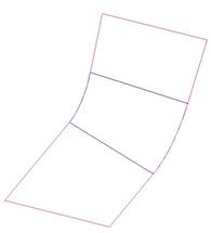
The last thing we can define in a boundary blended surface is any control points.  To demonstrate how this might make a difference, we will open up the Boundary3.prt file, which looks like the following.

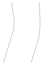
We will create a boundary blended surface by selecting the left curve and the right curves in the first direction.  The initial surface will look like the following.

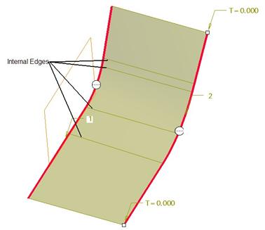
We can see from the figure above that Pro/ENGINEER must create internal surface edges to blend these two curves together.  This isn’t necessarily a bad thing, but the more internal surface edges you have, the less smooth the blend will be.  If we were to perform a full preview, and rotate the model, you would see shadows all across this surface, indicating high and low spots.  These spots occur where the internal surface edges are.

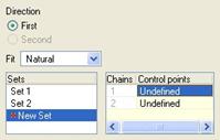
We will try to reduce the number of internal edges, thus performing a better blend.  To start, we will open up the Control Points slide-up panel, which looks like the figure below.

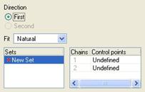
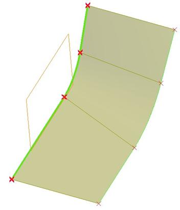
In the Sets section, we can see that we are defining a control point set.  In the field to the right, we will pick on the top-most Undefined.  When we do this, our model will highlight the first curve we selected, and place red “X’s” where there are internal vertices, as shown below.

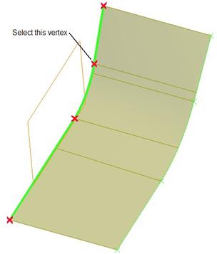
We can see four vertices, but only two of them are internal to the first curve.  We aren’t going to worry about the outside points, because they connect directly up to the endpoints on the second curve.

We are asked to select one of the vertices from this first curve.  We will select the topmost internal vertex, as indicated in the figure above.  When we do this, the second curve will now highlight with its internal vertices.

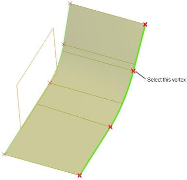
We will select the vertex on the second curve that is approximately opposite the one we just selected on the first curve (as shown in the previous figure).  When we do this, the top two internal edges become a single internal edge connecting the two, and we can now pick a second set of points, starting with the vertex shown below.

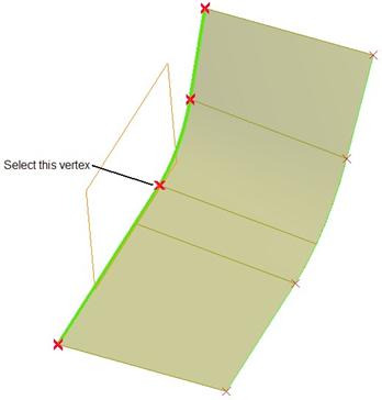
Once we pick the first vertex for the second set, the second curve will highlight, and we will pick the corresponding point on this edge, as shown below.

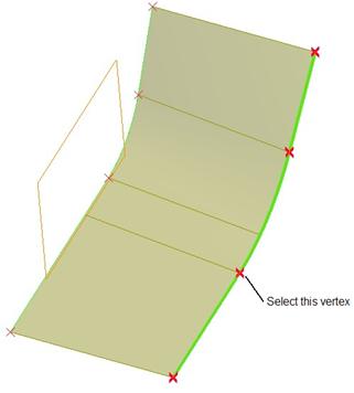
When we do this, we will see the bottom two internal edges replaced by a single internal edge, as shown in the next figure.

We do not have any additional internal curve vertices to select, and our Control Points panel looks like the following.

We will finish out of this boundary blend surface, and our model will now look like the following.

CURVATURE CHECK

Under Analysis, Geometry, Shaded Curvature, we have the ability to select all three surface pieces to perform a Gaussian curvature check.

If we were to perform a Gaussian curvature analysis on the original surface before we added the control points, and compare that to the same analysis on the newly reformed surface, we would see a big difference in the smoothness, as shown in the following two figures.

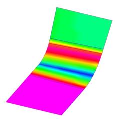
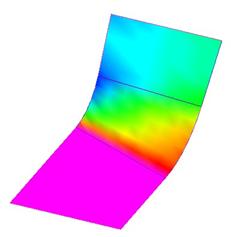
ORIGINAL SURFACE                                        NEW SURFACE

As we can see, there are ups and downs in the curvature of the first surface (it goes from magenta to red to green to blue to green again to yellow to red again to yellow again then to green again).

In the second surface, there is a continuous curvature change (it goes from magenta to red to yellow to green to blue).

This is a much cleaner and smoother surface, and will result in a more appealing product when light shines on it.

LESSON SUMMARY

Use a boundary blended surface to create a single surface connecting curves in one or two directions.  Use or create internal curves to help define the shape between the boundaries.

Always be aware of existing boundary conditions.  You want to make sure you are normal or tangent to entities that touch the surface to give you the smoothes transition.  Try to reduce the number of internal edges that result from the blend by using control points.  The fewer the edges, the smoother the surface will be.

EXERCISES

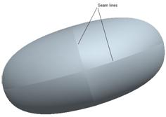
Open up the Boundary4 part file and turn shading on.  Notice that our surface does not look smooth across the center.  It has seam lines.

The model tree for this part looks like the following:

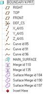
We will need to edit the definition of the feature called MAIN_SURFACE and adjust boundary conditions.  HINT: Since this surface was created by itself, then the model was mirrored twice to form the full part, you will not be able to use tangent.  Try one of the other boundary conditions.

The final result should look like the following.