Lesson

10

Lesson Objective: In this lesson, we will learn about Datum Curves.

DATUM CURVE USAGE

Datum curves are used in a wide range of applications.  They can be the trajectory for a sweep, variable section sweep or swept blend.  They can also be the boundary edges for blended surfaces.

They are often used as tools to create or modify surfaces.  We are going to learn about a variety of methods for creating datum curves.  We have already learned how to create a sketch feature, which produces a 2D curve on a plane or planar surface.  We will now look at the other types of datum features and tools.

PROJECTED DATUM CURVES

A projected datum curve is made by projecting a sketch or existing datum curve onto a nearby set of surfaces.  You can either project normal to the sketch or normal to the surface.  We will demonstrate both of these options, and discuss what is happening when you do this.

We will start by looking at the following part (Dtm_Curve1).

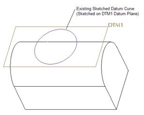
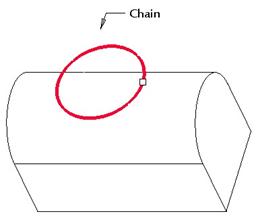
This part has a sketch feature on a datum plane (DTM1) that lies above the cylindrical surface, as we can see above.  We will use this curve to project down onto the cylindrical surface.

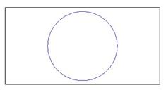
From a TOP view, we can see this circular datum curve takes up most of the width of the cylindrical surface, as shown below.

Therefore, we click on the Project Tool icon, as shown below.

When the dashboard opens, we will click on the References slide-up panel to see all of the options, as shown in the following figure.

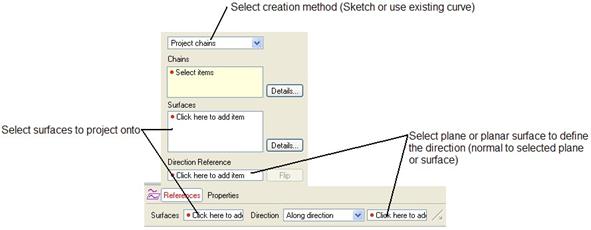
At the very top, there is a pull-down field.  Use this field to specify whether we are projecting an existing datum curve (Project chains), or whether we are going to sketch (Project a Sketch).  If we were to select the Project a Sketch option, our panel would look like the following.

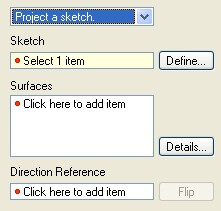
We can see a Define button that will allow us to go in and sketch the profile to project.  Instead, we are going to continue with the Project chains option.  Therefore, we need to select the existing edges or curves to project.  We will select the circular sketch that is already in the model. 

When we select it, it becomes a bold red, as shown in the figure at the top of the next page.

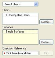
The References panel looks like the following.

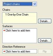
In the Chains field, we can see that “1 One-by-One Chain” is listed.  Now, we must pick the surface(s) we are going to project onto.  To initiate this selection, we can either pick in the next field down in the panel, or pick in the first field in the lower portion of the dashboard.  We will select the cylindrical surface, as shown below.

Our panel now shows this surface listed in the Surfaces field, as we can see in the next figure.

Now we come to the part where we pick to project from the sketching plane, or whether we will project normal to a surface.  Our two options are shown in the following figure.

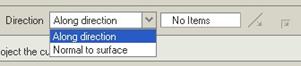
If we choose Along direction, then we must specify a plane or planar surface that the normal direction is based on.  If we choose Normal to surface we will not have to specify this.  We will select the “Along Direction” option and then pick the DTM1 datum plane.

The following figure shows the dynamic preview for the Along Direction with the DTM1 plane selected as the reference.

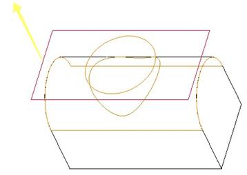
NOTE: The arrow doesn’t seem to make a difference in this case.  You could try flipping it, but it does not change the preview.

If we accept this result, from a TOP view, this is what we would see.

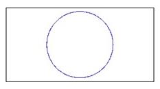
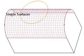
The projected curve is in exact alignment with the original sketched datum curve.  If we were to select Normal to Surface, our result would be the following.

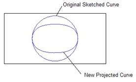
We notice that the projected curve is now more of an ellipse than a circle.  Why?

The reason is simple.  If we look at the following figure, we will see the answer.

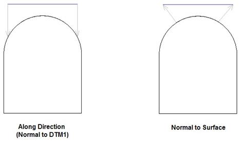
When you use Along Direction, the curve is almost extruded down onto the cylindrical surface, and the intersection of this imaginary extrusion and the surface creates the projected curve.

When you use Normal to Surface, the surface takes control of the projection.  It tries to locate the spot on the cylindrical surface that, when projected normal to the surface from that spot, it intersects with the original curve.  We can see that, due to the curvature of the surface, it actually starts up higher and in more to get to the same original circular curve.

In many cases, you may have problems getting a “Normal to Surface” projected curve to work unless you really understand what is going on with the way it projects.  Hopefully this will help you in getting the hang of it.

THROUGH POINTS

The next type of datum curve we are going to show is the Through Points (or in Pro/ENGINEER – it is spelled “Thru Points”).  This is a curve that passes through datum points or vertices.

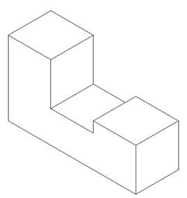
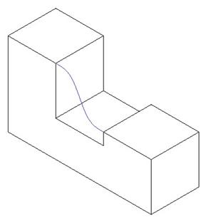
We are going to work with the following part (Dtm_Curve2) for this demonstration.

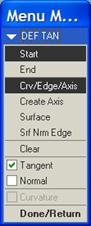
To create this curve, click on the general curve icon.  It brings up a set of menus called the Menu Manager, which looks like the following.

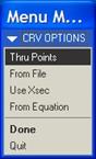
The first option on this list is the Thru Points curve, which is the one we want.  In the menu manager, you generally pick options at the top of the menu, then select Done, Done Sel or Done/Return at the bottom to continue.

In this case, since the Thru Points menu item is already selected (shown in a black highlight), we will pick on Done to continue.  This brings up the CURVE: Thru Points window, which looks like the following.

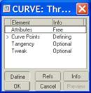
This is a different feature window than the dashboard.  Many of the more advanced features still use this type of window.  In the first column, entitled Elements, there is a list of items that we can define.

The second column, entitled Info describes what is happening or what needs to happen to the element in the first column.  You can see that we are currently defining the curve points.  Below this window, we can see more menus, that look like the following.

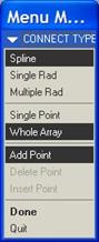
In the top portion, we define the way it handles corners (at the points along the curve).  If we use Spline, we get a continuous curve that is tangent along its entire length.  If we use Single Rad, then we will specify a single bend radius that it will apply at each corner.  If we select Multiple Rad, then we will be prompted to enter the bend radius at each point we select.

In this example, we are going to stay with the default choice of Spline.  In the second set of options, we can select Single Point if we want to pick individual points, even if they all belong to the same datum point feature.  If we pick Whole Array, then we will get all of the points in the datum point feature.  Since we are only going to go between to vertices, we won’t care what option it uses here.

Finally, we have one last section of this menu.  There is only one choice at this time, and that is to Add Points.

Down below this menu manager, we see another little window, which looks like the figure below.

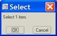
You are going to see this a lot.  Every time you are prompted to select something, this window will appear.  When you are finished selecting items, you click on OK to finish selecting.  The easier thing to do, however, is to use the middle mouse button to click once to indicate that you are finished.  It is the same as clicking OK.

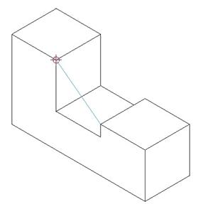
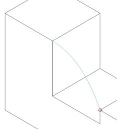
We are going to pick on the two vertices, shown in the figure below.

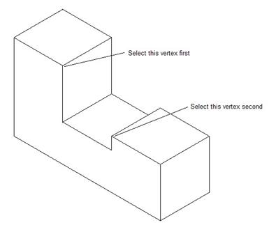
Once we select the second vertex, a blue arrow will appear, indicating the start point of the curve, as shown below.

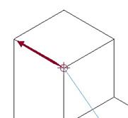
Since we are done selecting, we will click with the middle mouse button, then select Done from the menu manager.  We are now placed back into the CURVE: Thru Points window.  We are technically done defining all of the required elements.  There are still two optional elements we can define.  We will double-click on Tangency from the element list, which will bring up the menu manager shown at the top of the next page.

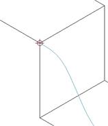
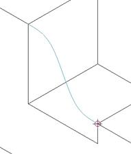
Looking at the menu above, we are asked to pick a Curve, Edge or Axis that defines the tangency for the start of our curve.  On our model, the start point is highlighted with a red circle, as shown below.

We will pick the edge at the top of the front surface that intersects this start point.  When we do, we will see the following on the model.

At the bottom of the menu manager, we see two options: Flip or Okay.  The arrow points towards the direction that tangency is measured from.  Many times, you will get it right the first time, and many times you will have to try again.

If we pick Okay at this point (with the arrow going away from the curve that we are creating), we will get the following.

This is one of the times that we got it wrong.  Not to worry, however.  All we need to do is pick on the Start menu item, pick the edge again, and this time flip the arrow, then click on Okay.  The result from doing it over looks like the following.

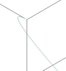
That is much better.  Once we define the start point, it automatically jumps to defining the End point.  We will pick on its adjacent edge, and flip the arrow so it is pointing in the direction shown at the top of the next page.

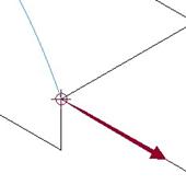
Once it is flipped to face in this direction, click on Okay to finish it.  The curve now looks like the following.

This looks pretty good – much better than the straight line we had originally.  Now that we have finished defining the references at each end for the tangency condition, we are placed back at the start point, and a new menu item appears in the menu manager, called Curvature. 

If we select this, the curve will take on the curvature of the entity that acted as the tangency reference.  Since our entity was a straight edge, our curve will receive a small straight portion to it at that end. 

The figure at the top of the next page shows what would happen if we selected Curvature for the start point.

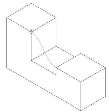
If we click on the end point, and select Curvature for this end as well, we get the following curve.

This is an even better curve, because it creates a smoother transition into the existing edges.  If we were to use this curve to create a surface between the two protrusions, then our surface would have very good continuity with the surrounding surfaces.

We are done defining tangency conditions, so we can select Done/Return at the bottom of the menu manager.  We are placed once again into the CURVE: Thru Points window.  We can see one last optional element, called Tweak.  If we double-click on this element, we see the following window.

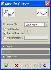
The curve on our model will show a control curve overlaid on it, as we can see below.

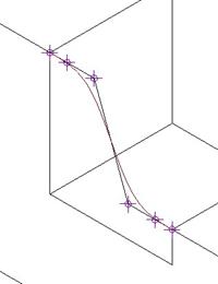
Using this menu, and/or dragging the control points on the model, we can adjust our curvature even more, or shorten/lengthen the straight portion of the curve as it goes into the adjacent edges. 

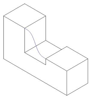
This basically gives us more control to Tweak the shape of our curve.  We are going to cancel out of this tweak window by clicking on the red “X” in the lower left corner.  Back in our CURVE: Thru Points window, click on OK to finish this feature.

The resulting datum curve will look like the following.

USE CROSS-SECTION

We haven’t talked about creating cross-sections yet, so we’ll just go into a part that already has one.  The “Use Cross-Section Datum Curve” creates a curve that represents the boundary of the entire cross section.

These curves are very useful for rib features, or other features that need a sketching reference but the shape of the surrounding geometry does not allow for picking as a sketcher reference.  The curve segments at this area are always selectable.

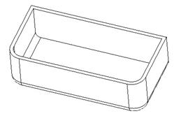
To demonstrate this, we will go back to a model that we saw in Lesson 3 – Selecting Objects (Selecting.prt).  When we open it, it looks like the following.

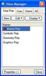
To access the cross-section functionality, go to View, View Manager from the menu bar.  We will get the following window.

Click on the Xsec tab at the top to get to Cross-section functionality.  The window will now look like the following figure.

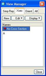
In this window, we can see a cross-section that already exists, called A.  If your section is not visible on the model, click on the A row in the main window.  The cross section looks like the following on the model when it is visible.

Now, we can close out of this window (which will make the cross-section disappear from the model), and create our curve.

To create a cross-section datum curve, click on the General Curve tool.  When the menu appears in the upper right corner of the screen, select Use Xsec, followed by Done.  The menu will list all of the available cross-sections in the model, as shown below.

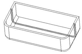
We can see the cross section “A” that we just looked at a minute ago.  When we select A from this list, the curve is automatically created, as shown below.

The curve takes on any external edge that the cross-section goes through.  That is why it goes around the entire part.

COPY CURVE (COMPOSITE)

There are many times when you will need to have a single curve defined.  A trajectory for a sweep might be a great example.  However, many times you are unable to create a single curve that captures what you want.

Therefore, you create multiple curves, and then you need a way to splice them all together to form a single curve.  This is where the Copy Curve comes in.

With this curve tool, you can select from existing edges or datum curves to form a single curve.  To demonstrate this, go back to the Dtm_Curve2 model that we just worked with.

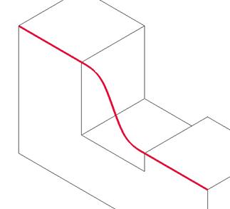
In this example, we want to create a single curve using the following three edges.

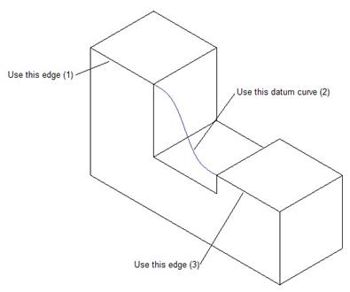
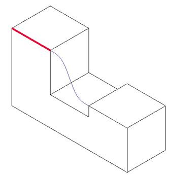
To create the copy curve, we first need to select the entities.  Therefore, we will make sure our Smart filter is turned on, and we’ll begin by selecting the solid protrusion so it highlights in red.  While this protrusion is highlighted, move your mouse over to the edge labeled (1) in the figure above and select it.  It should be bold, as shown in the following figure.

Something unique to the copy curve feature is the fact that we can NOT hold down the CTRL key and pick the other two entities.  We must first hold down the SHIFT key on the keyboard, then RE-SELECT the same edge that we already selected.

Once that edge is selected, keep the SHIFT key pressed and pick the other two entities.  They should all be bold, as shown below.

Now that all of our edges are selected, we will go to Edit, Copy from the menu bar (or select Ctrl-C on your keyboard).  Next, use Edit, Paste from the menu bar (or select Ctrl-V on your keyboard).

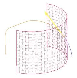
When we do this, our model will look like the following.

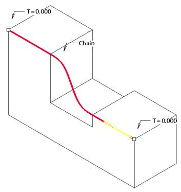
There is a yellow arrow at one of the endpoints (in this case the right-most end), which indicates the start point for the newly created curve.  The little “T” symbols at the ends represent the distance away from the end that we want to end the curve.  A value "0.00" will cause it to be at the exact length of the original geometry.  Any value other than 0.0 will cause the curve to extend beyond the geometry or end before the vertex. 

The default value is 0.000, which assumes that the new curve takes on the exact length of the existing curves/edges.

The dashboard for this copy command looks like the following.

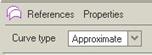
In the Curve Type field, we have two choices.  They are:

· Exact – The new curve takes on the exact shape of the selected entities.

· Approximate – The new curve creates a C2 Continuous curvature condition from existing C1 continuous entities.

The only potential problem with the “Approximate” option is that the new curve may “liftoff” from the existing curves.  The “Exact” option will keep the original curves as they are.  The only restriction with using the “Approximate” option is that the curves already have to be tangent.  Exact will allow you to use non-tangent entities. 

Therefore, we will change the Curve Type to Exact, and then accept this feature.  The following figure shows the resulting curve in our model.

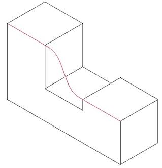
The curve may be difficult to see that it extends into the existing edges, but if you pick on it from the model tree to see it highlight, then you will see the figure above.

INTERSECT SURFACES

Another curve type is created by the intersection of two surfaces.  To demonstrate this, look at the following surface model (Dtm_Curve3).

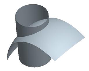
We will make a datum curve at the intersection of these two surfaces.  Therefore, we will begin by changing our selection filter to Quilts, and then pick the cylindrical surface, followed by the revolved surface.

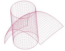
The figure below shows both of these surfaces selected (in No Hidden viewing mode).

Once both surfaces are selected, we will pick on the Intersect icon in the feature toolbar, which looks like the following.

NOTE: There are three icons in the feature toolbar that look very similar.  These are:

·  Merge – Merges two surfaces together to form a single quilt.

· Trim – Uses a surface or a curve as a trimming tool to act on another surface or curve.

·  Intersect – Intersects two surfaces to form a datum curve, as we see in this lesson.

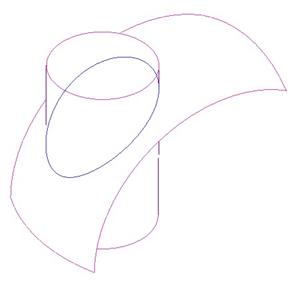
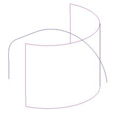
Be sure you are grabbing the correct one.  Once we select on the Intersect tool, the datum curve should be created automatically, as shown in the following figure.

TRIM CURVE

Another operation that can be performed to create a new curve is to trim the curve using another curve or surface as the trimming tool.  In this example, we will use a surface as a trimming tool.

Look at the following model (Dtm_Curve4).

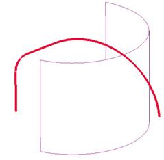
We are going to use the surface as a cutting tool to remove the portion of the curve that sticks out to the right of it.

When creating a trim curve feature, always start by selecting on the object that you are trimming, in this case the curve.  Use the Smart filter to select the curve, as shown below.  NOTE: If the curve is made of multiple segments, as it is in this case, you will need to pick on the part of the curve that is being trimmed.

Once you have the curve selected, pick on the trim icon, as shown below.

When we enter this feature, we will click on the References slide-up panel in the dashboard to see the different entities we are selecting.  It will look like the following figure.

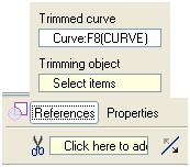
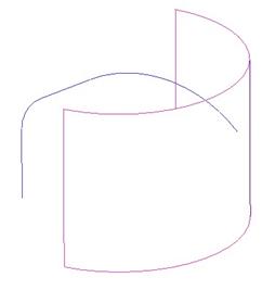
We can see that the curve we selected shows up in the Trimmed Curve field.  We are prompted to select the Trimming object.  We will pick on the extruded surface.  Our model now looks like the following.

An arrow appears at the cut location, and points towards the part of the curve that we want to keep.  Flip the arrow if it is not pointing in the correct direction.  Once you approve of the cutting direction, click on the green check mark to accept this.  The curve will be trimmed up to the surface, as we can see in the following figure.

LESSON SUMMARY

Datum curves are very useful tools for creating other datum features, surfaces or solid geometry.  There are a variety of tools available for creating or editing curves.

The most common curve types are sketched and projected.  Remember that with the projected curve, normal to surface may give you results that you do not expect.

EXERCISES

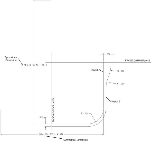
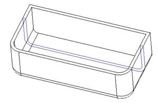
Create a new part called Basket, and create the two sketched curves (as individual curve features) that you see below (complete with dimensions).  Create these on the TOP datum plane as the sketching plane.