|

Lesson Objective: In this lesson, we will learn about the 6DOF connection type.

USAGE OF 6DOF
There are times in an assembly definition, when you need to leave a component completely free to translate and rotate in any direction. Normally, you might consider just leaving a component unplaced, but then no other components will react with it. Therefore, this connection type will allow you to define this type of freedom, but still tie it into the assembly using a datum coordinate system.
EXAMPLE – BOUNCING BALL IN CUBE
We are going to simulate a ball bouncing in an enclosed cube where all the collisions between the ball and the cube walls are perfectly elastic. Therefore, we are going to start by opening up the assembly called 6DOF_ASSY, which initially looks like the following.
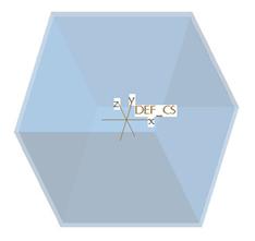
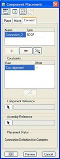
Currently this assembly consists of a transparent cube. We will now assemble in the 6DOF_Ball component. When we get to the assemble component window, we will click on the Connect tab to define mechanism connections. Change the connection type to 6DOF. The window will now look like the following.
Select the coordinate system on the ball and the coordinate system on the cube, then select OK to complete this connection. Go to Applications, Mechanism and you will see the connection, as shown in the next figure.
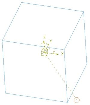
We can see a straight and curved arrow for the x, y and z axes. We are now going to set the zero location and limits for this ball.
Joint Axis Settings
We will start by query selecting until we get the straight arrow for the “X” direction. Once you have that arrow selected, right click and go to Joint Settings. When the joint settings window appears, we will click on the Regen Value tab and check the box to regenerate at 0. The “0” location for all three axes should set the ball at the center of the cube.
Once you have turned on the regeneration of the ball at “0”, click on the Properties tab, enable limits, and set the following:
Minimum Limit: -5.5
Maximum Limit: 5.5
Coefficient of Restitution (e): 1.0
Joint Axis Position: 0.0
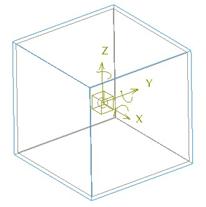
Repeat this process for the “Y” and “Z” axis as well. The ball should snap to the center of the cube, as shown in the next figure.
So, why did we set the limits and coefficient of restitution? We might be tempted to set up cams to stop the ball at the inner walls of the cube, but we won’t be able to. A limit of cams is that you can not use “spherical” surfaces as cam surfaces. Only planar or cylindrical surfaces will work for cams. Therefore, we use the limits (6 inches from the center of the cube to any wall – minus ½” for the radius of the sphere) to define the maximum travel for each axis.
The coefficient of restitution at 1.0 defines an elastic condition at the limits of the ball travel. This way, when the ball reaches one of its limits in an analysis, it will elastically bounce back the other direction.
We will not have any servo motors defined for this analysis, because the ball’s travel is not going to be in any one particular direction.
Initial Conditions
Once you have the ball sitting at the center of the cube, we
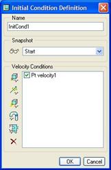
will define a snapshot called Start. Once you have your snapshot
defined, click on the define initial conditions tool ( ![]() ). When this window comes up,
select the snapshot, as shown in the next figure, but do not close out of this
window.
). When this window comes up,
select the snapshot, as shown in the next figure, but do not close out of this
window.
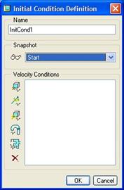
Down the left side of this window, there are some additional icons. These icons are:
· Define velocity of a point
· Define joint axis velocity
· Define angular velocity
· Define tangential slot velocity
· Evaluate model with velocity conditions
· Delete highlighted condition
We will select the Define Velocity of a Point icon, and select the datum point at the center of the ball, which brings up the following window.
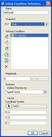
The first thing we are going to do is use the arrow button to select the DEF_CS coordinate system of the ball model. Be sure to use Query Select to get the one with the ball, as both the ball and cube are right on top of each other.
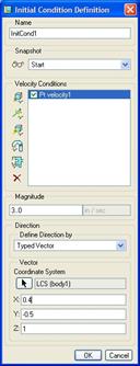
Next, enter a magnitude of 3.0 in/sec in the field provided. Finally, we are going to define the vector values for the force. Use the following:
X: 0.4
Y: -0.5
Z: 1.0
Our window should now look like the following.
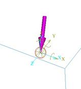
On the model, we can see a magenta arrow indicating the direction of the applied force, as shown in the next figure.
Click on OK to complete the velocity definition, and our initial condition window looks like the following figure.
What we are doing here is saying that when the analysis starts, the ball is going to be traveling at 3 in/sec in the direction specified by our vector. Where the ball goes from here is all up to the conditions in the assembly (mostly the joint axis settings in this case). Click on OK to close this window, followed by Close to complete defining initial conditions.
Analysis
We will now define a new Dynamic analysis. Be sure to set the initial condition at the bottom of the first screen, and change the analysis time to 60 seconds. There are no motors, and we will not enable gravity or friction to start.
Run the analysis, and you should see the ball bouncing off the inner walls of the cube. To see a captured movie for this motion, open up the 6dof_motion.mpg movie in your training directory.
LESSON SUMMARY
Use a 6DOF connection to simulate an object that has a completely open set of translations and rotations. You may need to be creative in defining joint axis settings and initial conditions to simulate motion for the object if it is not tied to any other object.
EXERCISE
Continue with this same assembly and create a trace curve for the ball at the current settings. Next, try changing the coefficient of restitution to a more plastic value (0.3, for example) and see how this affects things.
Save and close your assembly when done.